

Primer
When the H100 shipped in 2022, analysts expected it to be obsolete long before the six-year depreciation schedules that hyperscalers book for their servers. Today, it seems the opposite has happened. H100 rental prices climbed through 2026, with SemiAnalysis's one-year reserved index up about 40% from its October 2025 low, and H100s whose original 2022 contracts expired at CoreWeave were rebooked at 95% of their original price. In fact, they remain a crucial component of the stack for inference providers who meet strict latency and throughput SLAs.
On the other hand, open weights models are getting larger. In early 2025, the largest open weights model held around 670 billion parameters (DeepSeek V3). Today, Kimi K3 holds 2.8 trillion, more than quadrupling the RAM and HBM requirements to serve a SOTA open-weights LLM. Syzygy's thesis is that two things can be true: the H100 will remain a powerful machine for inference over the remainder of its useful life, and trillion parameter LLMs will become the standard for frontier open weights inference. This is true because we find that it is not the number of bytes required to represent the LLM that scales with performance, but rather the number of parameters. By reducing the bytes per parameter while maintaining quality, we can extend the useful life of non-frontier GPUs significantly, providing both consumers and datacenters lasting value on their purchased devices. Of course, by slashing memory requirements, we can also achieve significantly faster latency and throughput at decode time on equivalent hardware.
This post highlights the two common alternative representations of floating point LLM weights, and discusses a new approach that pushes the bits (perplexity)-per-byte (per LLM weight) frontier while boosting inference speed. While at decode time inference is primarily memory-bound, these advantages can be subsumed by compute latency if the codec, or representation of the weights before computation, requires many instructions to decode weights into floating point format. Thus, we discuss methods for constraining codec design to reduce additional arithmetic at inference time.
Scalar representations are what we all know and love, and they represent the vast majority of inference today because they require little to no additional arithmetic to perform matrix multiplications with. Vector representations, as we shall discuss, must decode into a vector of weights before inference, but tile the space of possible rounding (or quantization) options for groups of weights more tightly than scalar. Trellis representations share bits between weights, reducing memory requirements further. We introduce the spherical trellis, a trellis that decodes into the densest sphere-packing, or vector, lattice in four dimensions. Finally, we will discuss how to reduce the arithmetic required to decode a complex codec like the spherical trellis and thus better utilize the High Bandwidth Memory (HBM) at decode time.
Scalar quantization
Scalar quantization is the simplest possible representation of an LLM in GPU memory. Floating point numbers described with up to 32 bits in precision describe each individual element of any matrix. Scalar quantization swaps each one for a short code. With 2 bits, you have 4 possible numbers for each position. With 4 bits, you have 16, and so on.
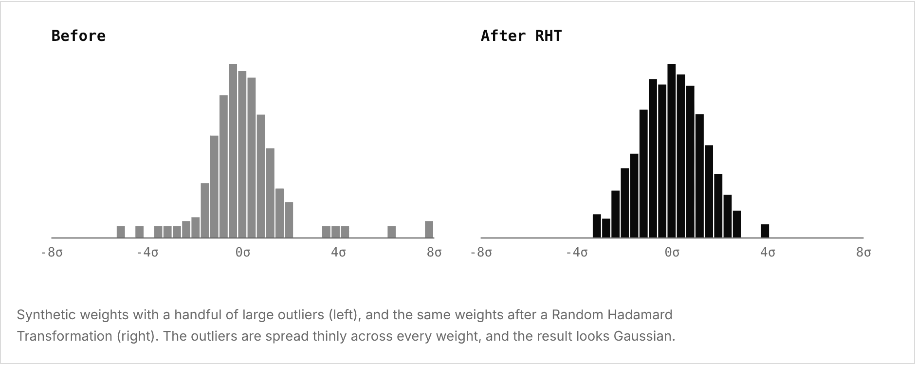
How do we decide what 4 levels to choose from in a weight matrix? Suppose ideal conditions, where every weight is 0, 1, -1, or 2. Then the answer is simple, we choose those 4 numbers. Now make it less than ideal, one weight has a value of 0.8. This is fine, we can simply round it to 1 and accept a small error. In fact we can choose our set of possible mapped weights (our codebook) so that the total error across the matrix is small. But suppose one weight has a value of 10, and all other weights have values between -1 and 1. In this case the error is large, and the overall computation may be completely thrown off by rounding. A simple and effective way to get around this is to transform our weights first so that they can decode to a fixed codebook without large outliers creating large errors. This can be done with a Random Hadamard Transformation, which makes our weight matrices look like they were from a Gaussian distribution. After we do our inference work, we can reverse the RHT to go back to the actual weights.
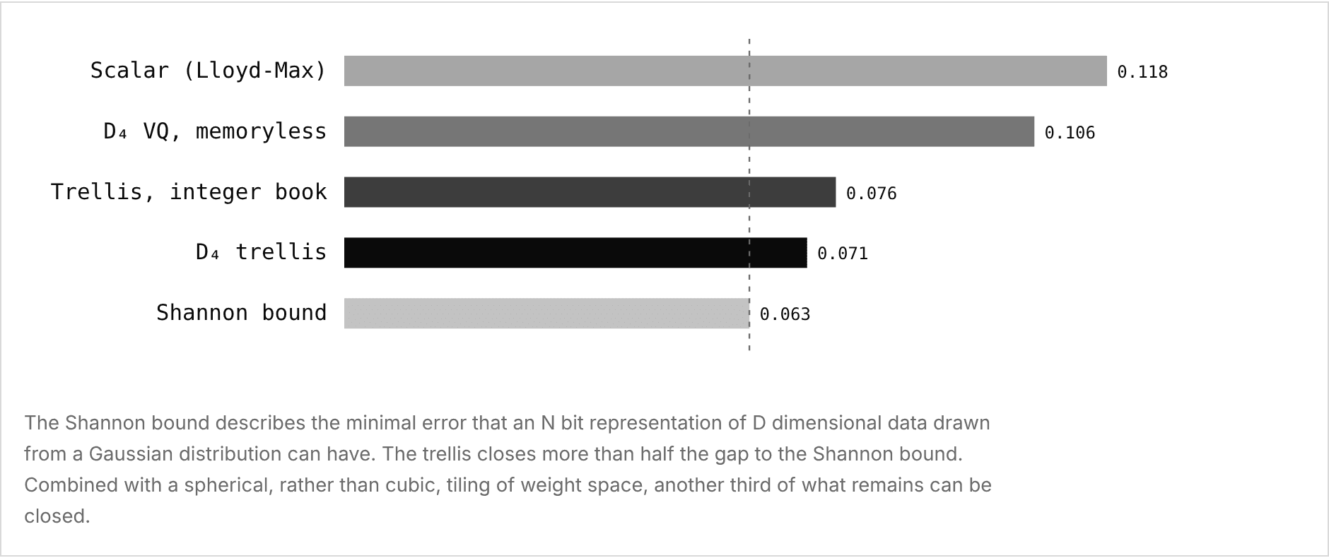
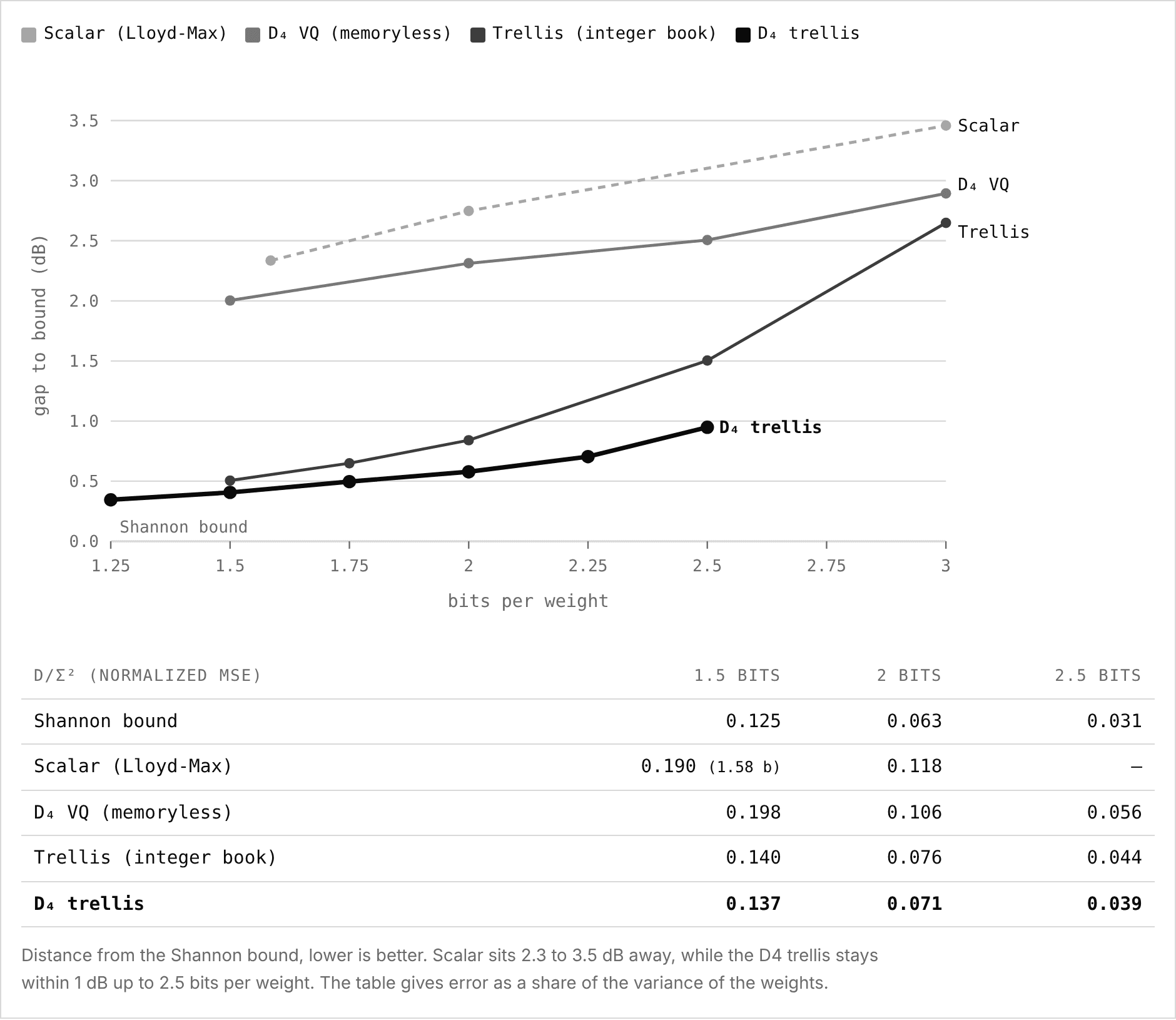
Even with the best possible choice of levels, scalar quantization leaves a lot on the table. Claude Shannon found that the minimal error for Gaussian data at R bits per weight is 2^(−2R) of the variance, which is 6.25% at 2 bits. The best 2-bit scalar codebook leaves 11.8%, almost double the bound. In fact, at 2 bits scalar quantization wastes close to half a bit on every weight, and the gap gets worse as you add bits. Ternary, the −1, 0, 1 codebook behind BitNet, shows the same idea at 1.58 bits.
Vector quantization
Now suppose that instead of rounding each weight on its own, we round two weights at a time. With 2 bits per weight, a pair of weights gets 16 possible values, the same as two scalar codebooks of 4 levels each. With scalar quantization those 16 points have to sit on a grid, so the regions that round to each point are rectangles. The average rounding error then scales with how densely we can pack codebook items into the region our Gaussian data consumes. A spherical grid can tile this region more densely than cubes, which is the motivation behind vector quantization.
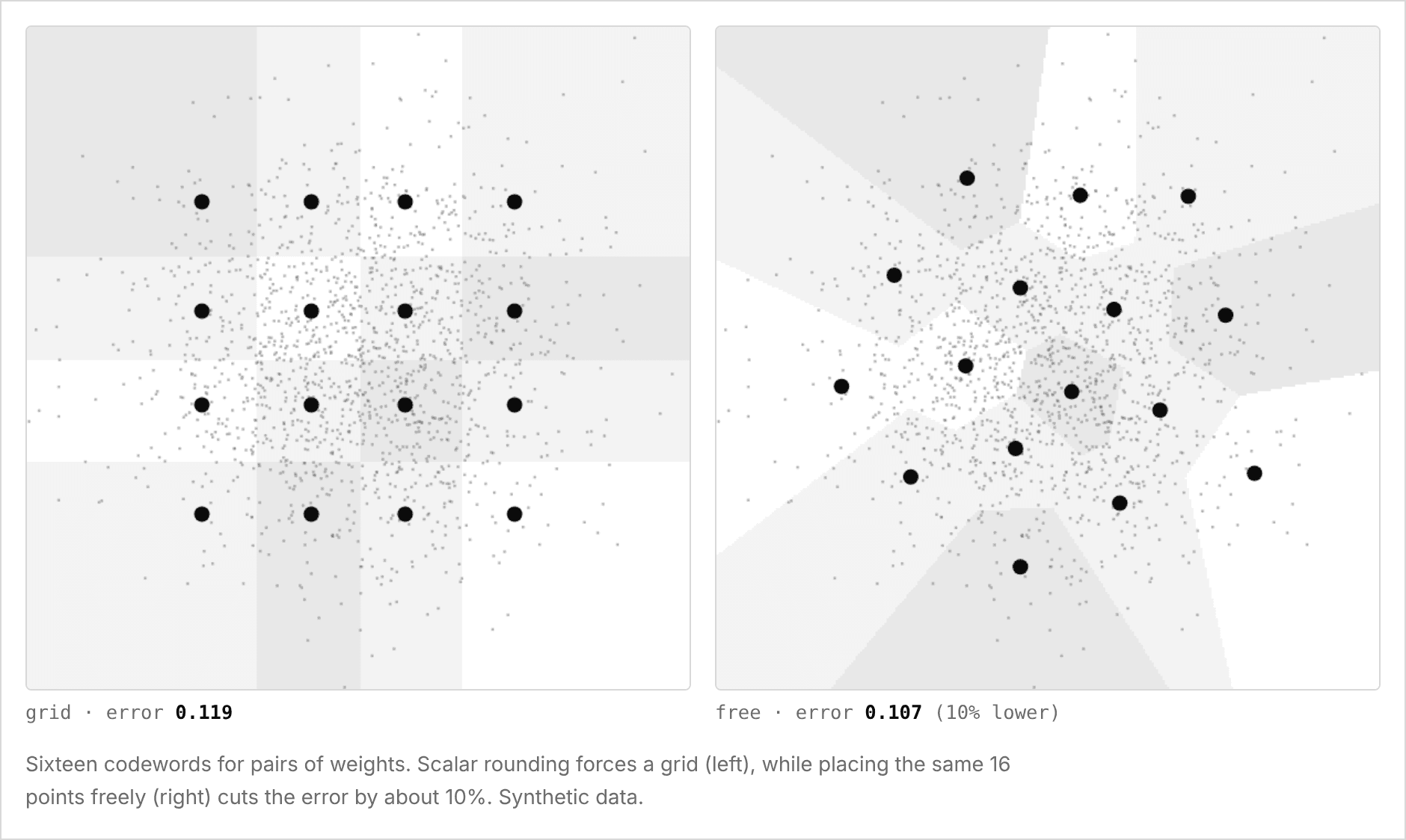
Why do rounder regions help? The largest errors in a cube come from its corners, and a sphere has no corners. So the search for the best vector codebook becomes an old question in geometry, how tightly can you pack spheres? In two dimensions the answer is the hexagonal grid of a honeycomb. In four dimensions it is a lattice called D4, which is every point with integer coordinates that add up to an even number.
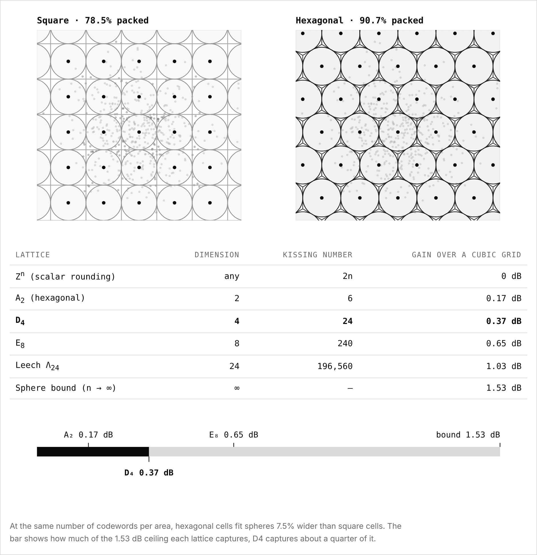
Thus vectors fix the geometry of our codebook, but each codeword is still chosen on its own, and neighboring weights have nothing to do with each other. What if they could share some of their bits?
Trellis quantization
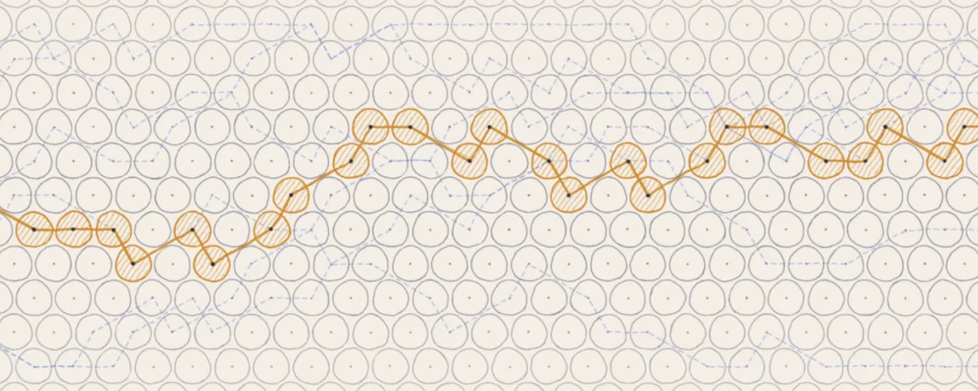
Picture the compressed weights as a tape of bits, with a window of 16 bits sliding along it. At each step the window moves forward by 6 bits, and the 16 bits inside the window pick the next 4 weights from a table. Since 10 of those 16 bits were already in the window at the last step, each codeword overlaps with the one before it. We allow for 6 new bits for every 4 weights, which is 1.5 bits per weight, and codewords are chosen from 65,536 options. This is the bitshift trellis from QTIP, and it is the base of our codec.
The downside is that we can no longer pick each codeword on its own, since choosing these 6 bits changes what the next two codewords can be. To search for the best tape we use the Viterbi algorithm, which walks along the tape and preserves only the cheapest way to arrive at each of the 65,536 window states. This is expensive, but we only do it once, when we compress the model. Decoding, on the other hand, is cheap, involving a shift, mask, and look up.
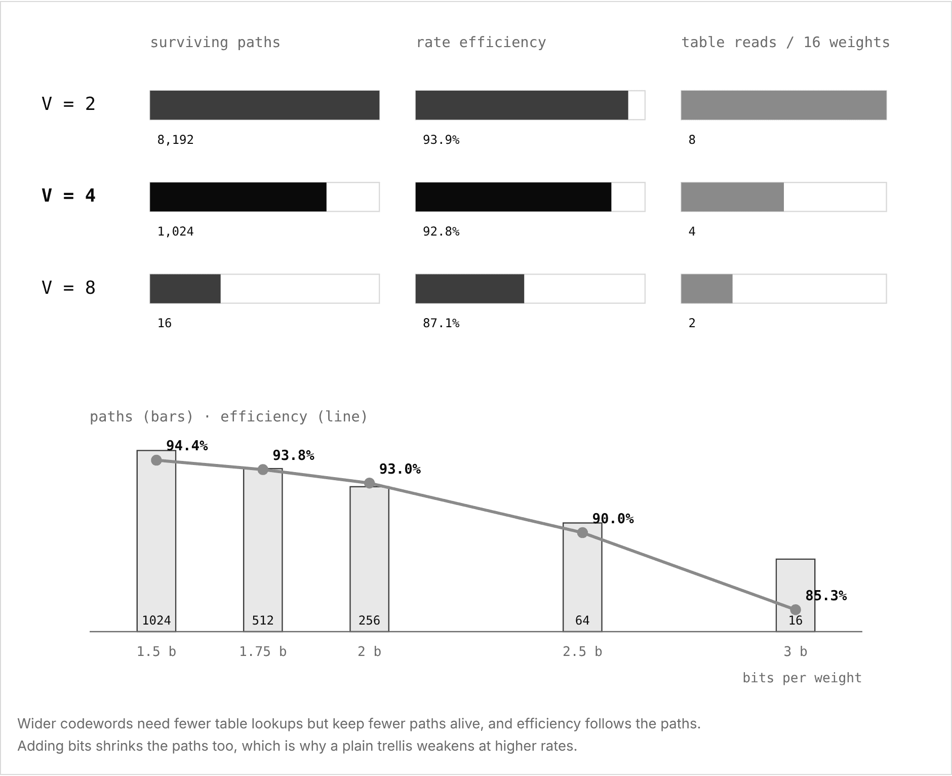
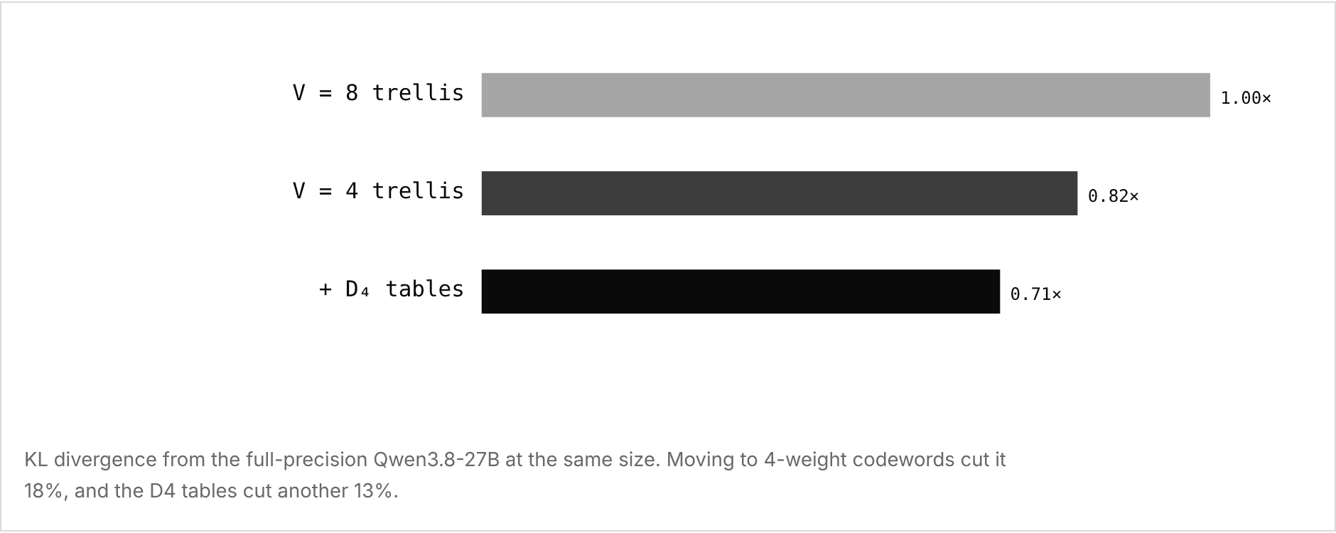
The quality of the trellis thus depends on how many paths it enables. With a 16-bit window that shifts in K·V bits per step (K bits per weight, V weights per codeword), there are 2^(16 − K·V) ways to arrive at each state. Our earlier codec packed 8 weights into every codeword, which at 1.5 bits per weight left only 16 paths. Switching to 4 weights per codeword creates 1,024 paths and improves our rate efficiency. On Qwen 3.8, this cut KL divergence by 18%.
The spherical trellis
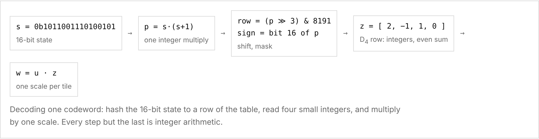
In the spherical trellis, every one of the 65,536 rows of the code table is a point on the D4 lattice, four small integers that add up to an even number, times one shared scale. The trellis shares bits between neighboring weights, while the lattice defines the geometry of the codeword.
We build the table as follows: first, we train it with no constraints, running the Viterbi encoder over Gaussian weights and shifting each row to the average of the weights it is intended to represent. Then we snap every row to its nearest point on the spherical lattice. The snap costs a negligible amount in error, allowing every codeword to become a short list of integers, and debiasing rounding errors.
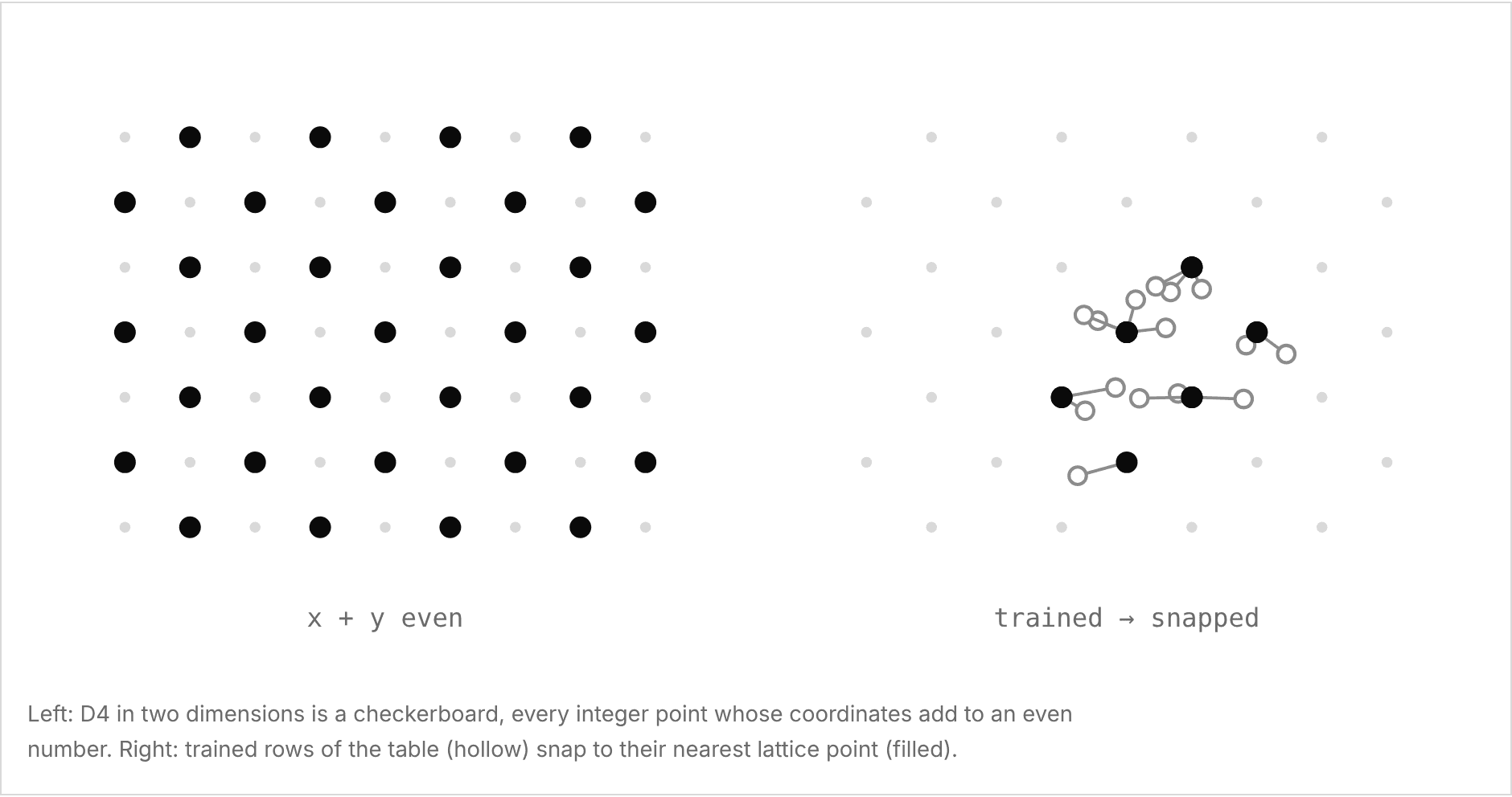
However, originally, a codebook made only of D4 points, with no training, did worse than our old codebook, and so did a classic trellis design built around D4. We found that snapping states to the lattice afterwards led to better performance at the same memory.
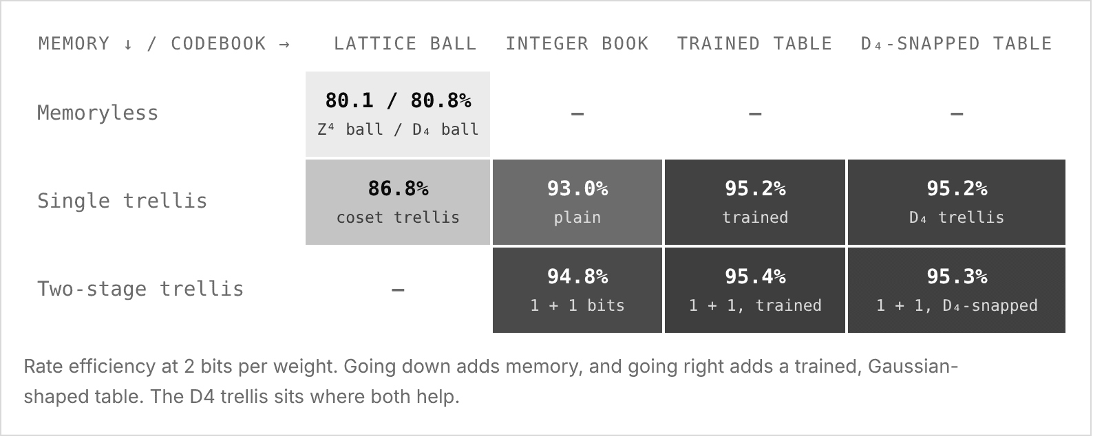
On Qwen3.8-27B, moving to the D4 table at the same size cut KL divergence by 13%. The snap mattered here for a reason MSE (mean squared error) does not show. Trained tables make errors that point the same way in every layer, and those errors pile up as they pass through the network. Snapping to the lattice cut that pile-up roughly in half.
The spherical trellis lets neighboring weights share bits through a 16-bit sliding window, and makes every codeword a trained point on the densest four-dimensional spherical lattice.
Constraining the codec for inference
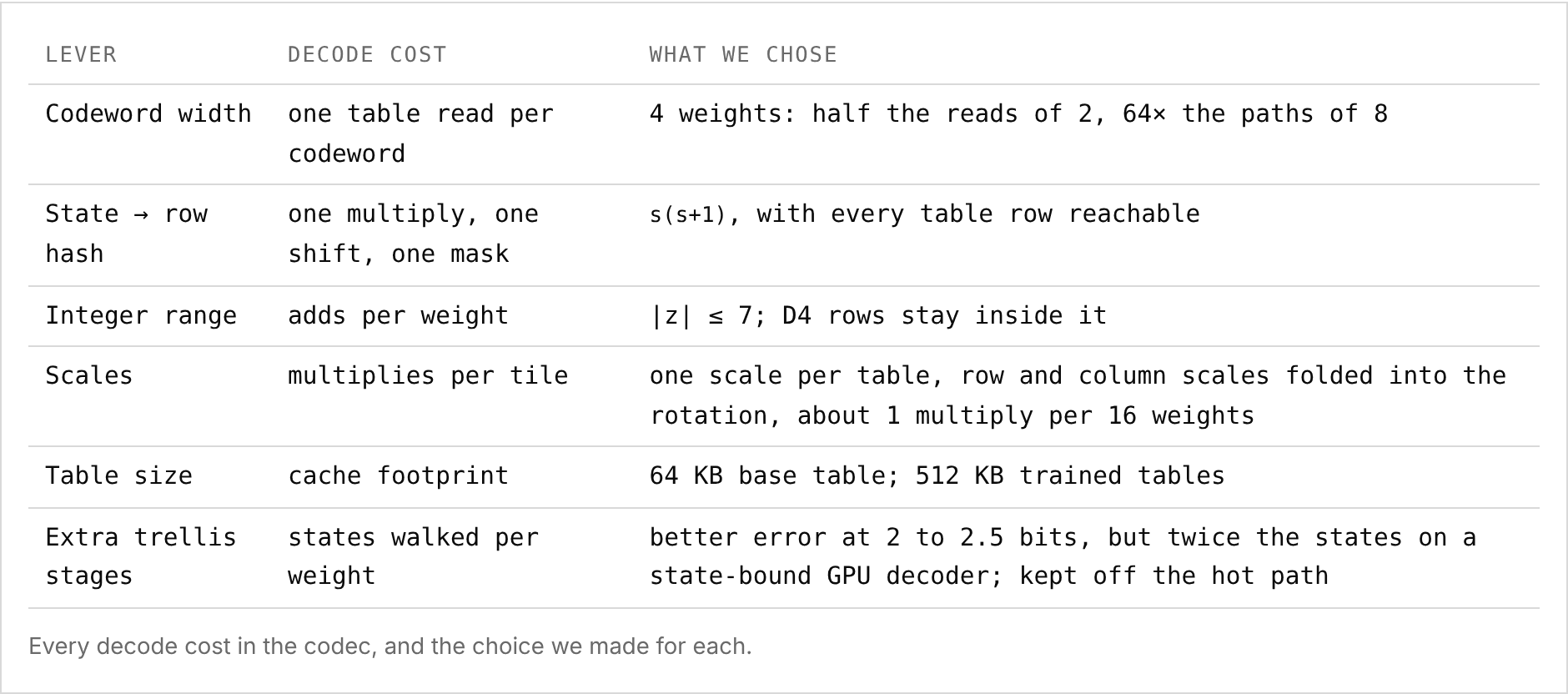
At decode time, a GPU spends most of its time waiting on memory, which is why fewer bytes per weight makes inference faster. However, this only holds if turning those bytes back into weights is cheap. If decoding takes too many instructions, the GPU stops being memory bound and is instead compute bound, and we lose our speedup. Thus, we hold the spherical trellis to two constraints: every codeword is additive, and the work per weight is small and predictable.
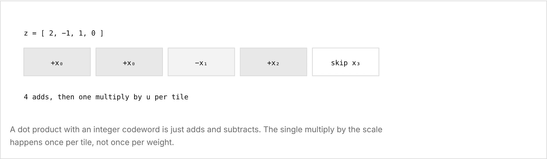
Additive means that every codeword is a list of small integers times one shared scale. Suppose the codeword is [2, −1, 1, 0] and the four activations are x0 to x3. Instead of four multiplies, the dot product is x0 + x0 − x1 + x2: add the first activation twice, subtract the second, add the third, and skip the fourth. The scale is applied once to the sum of the whole tile at the end. We cap every integer at 7 in absolute value so that the chain of adds always stays short.
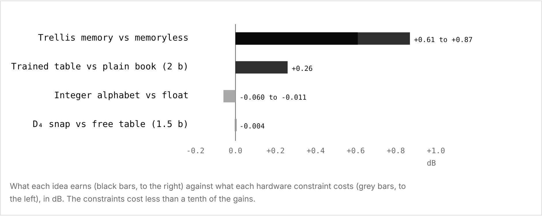
Compared with a floating point codebook inside the same trellis, integer codewords cost between 0.01 and 0.06 dB, while the trellis itself cuts 0.6 to 0.9 dB, and the D4 snap costs less than 0.01 dB. Mach runs every weight matrix multiplication with only adds and subtracts, at 1.7 bits per weight, and preserves nearly 100% of performance on long context evals like DeepSWE. Decoding without multiplies is important where arithmetic is scarce, like CPUs on phones and laptops.
The second constraint is instruction count. The width of each codeword is the clearest trade-off. Two weights per codeword compresses best, but needs a table lookup every two weights. Eight weights per codeword needs the fewest lookups, but drastically cuts the number of paths available to the trellis. Four sits in the middle, which is what we ship today.
Final Comparison
To compare codecs fairly, we encode the same 2 Gaussian numbers with every method. This is a stand-in for real Qwen weights after the Random Hadamard Transformation. We measure how far the error of each codec sits from the Shannon bound.
What comes next
Mach currently enables us to nearly losslessly run large open weights LLMs on fewer and less expensive GPUs, as well as personal devices. It also accelerates inference speed at decode time by moving around less memory. If you serve open weights models and want more out of the GPUs you already own, we would love to talk (dhruv@withsyzygy.com).
If you would like to test Mach 2 Medium or Mach 1 Small on a MacBook, head to our website at withsyzygy.com.
Relevant Links
Mach Cloud Waitlist: https://withsyzygy.com/inference
Native Format: https://huggingface.co/SyzygyResearch/Mach-2-Additive-Medium
GGUF: https://huggingface.co/SyzygyResearch/Mach-2-Additive-Medium-GGUF
llama.cpp: https://github.com/SyzygyResearch/llama.cpp-mach1
MacOS: https://withsyzygy.com
Notes and sources
H100 pricing. SemiAnalysis one-year reserved index ($1.70 → $2.35 per GPU-hour, Oct 2025 → Mar 2026) and CoreWeave rebooking at 95% of original pricing, as reported byThunder Compute, GetDeploying and Applied Conjectures. Six-year server depreciation: same Applied Conjectures piece and the CUBE Research.
Model sizes. DeepSeek V3 (671B, Dec 2024); Kimi K3 (2.8T) per Wikipedia and Layer3 Labs
Lattice gains. Conway & Sloane, Sphere Packings, Lattices and Groups.