

Gains for DeepSeek on B300s:
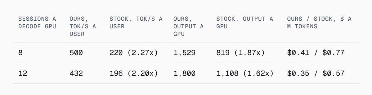
- 2.2–2.3× decode speed per user over stock vLLM
- 2.1–3.0× speed per user over the best stock setup at the same cost, 32 to 128 agent sessions
- 0.085 vs 0.13 KL added vs original model variance
1. Introduction
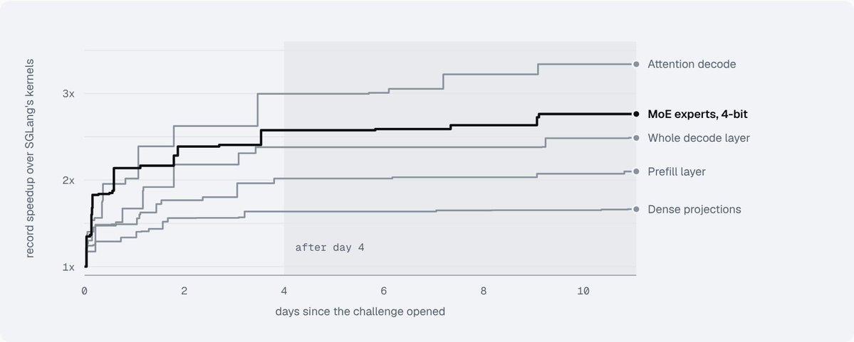
For large mixture of experts models such as DeepSeek, memory bandwidth is typically the primary constraint of the decode step of serving such models. Better kernels can help move closer to the memory bandwidth constraint of the server, but they approach the same fundamental limit. This is why in an open kernel challenge such as Muse Spark Open Kernel Challenge to beat SGLang’s kernels, the best results plateau after a few days.
Most of the time during a decode step for a mixture of experts model is spent waiting for the weights of the experts that the tokens of the step select to be read from memory. Thus, methods that read fewer bytes of weight for a token (such as Deja Vu, PowerInfer, LLM in a Flash and TEAL) must make a decision per token of whether to read any of the weights for that expert or not. Even if a batch of tokens contains many that select the same expert, the total number of bytes of weight that must be read for that expert is the union of the bytes of weight that must be read for each of the tokens in the batch.
The distribution of tokens in a step over the experts is not uniform. Some experts (and the GPUs where they are stored) will carry far more of the step than others. This load is typically evened out by serving systems (e.g. EPLB of DeepSeek) by moving and copying experts between GPUs. We can also even out the load of the weight reads by reading an expert deeply when many tokens use it and shallowly otherwise.
2. Decode primer
Notation. DeepSeek V4.1 Flash has 40 layers of 384 experts. Routers choose 6 experts for every token t with weights rₜ,ₑ. Each expert is a gated MLP with I hidden neurons. Neuron i has gate and up rows wᵢᵍ and wᵢᵘ, output weights wᵢ and activation hᵢ. F is the Fisher information of the next-token distribution with respect to a layer's output. 𝔼 averages over decode.
Storage. The experts of a mixture of experts model are typically stored in the original MXFP4 format of the model, with the neurons of each expert sorted by their importance in terms of the expert’s expected output energy, and grouped into tiles of size 64. Thus, reading the first Hₑ tiles of an expert as compression of that expert’s weights is just one contiguous read of HBM, and can be done at any desired precision, from a few tiles up to the full expert.
Cost of a step. The cost of a step is determined by the number of experts that a step reads and the number of tiles that a step reads of each of the experts that it reads:
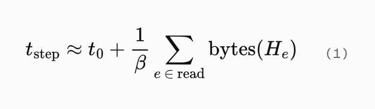
where β is the memory bandwidth and t₀ is the static portion of work. What a read is worth to the user and GPU owner, on the other hand, depends on how many tokens use it and how much weight the router gives them. For example, suppose a step decodes 16 tokens. Each token picks 6 experts, so the step makes 96 picks, which is mostly concentrated on a few experts with a long tail. A fixed-precision model reads every one of those experts in full. It spends as many bytes on an expert that one token uses with a small router weight as it does on an expert that many tokens share.
3. Why cut whole neurons?
An expert computes
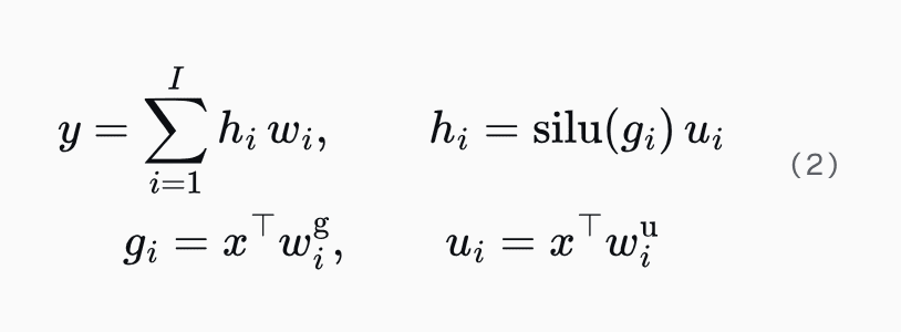
For a linear expert, the best way to cut it down to k directions is to do a whitened SVD by the Eckart Young theorem. However, the nonlinearity in Equation 2 acts on each neuron separately. This means that the only changes of basis that pass through the nonlinearity unchanged are permutations and rescalings of the neurons. Hence, cutting in any other basis would require first computing all of the hᵢ’s for the full expert, which in turn would require reading all of Wᵍ and Wᵘ for the full expert. Thus, the only cuts that save bytes are those that drop whole neurons.
Definition 1 (drop cost). The drop cost of neuron i is dᵢ = 𝔼[hᵢ²]‖wᵢ‖², its share of the expert's expected output energy.
Dropping a set S changes the output by −Σ_(i∈S) hᵢwᵢ, so its expected energy is the sum of the drop costs plus the cross terms between dropped neurons:
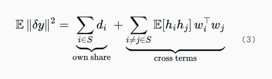
Since the cross terms are small, the best subset of any size consists of the neurons with the largest drop costs. Hence, we store the neurons of each expert in that order.
4. How much can we compress?
Note that the first-order term of the KL of a cut to the original model vanishes because the original model is a minimizer of the KL, so we only care about the second-order term of the KL for the next-token distribution with respect to a layer’s output for a cut to the original model. For a fixed-precision model, this is given by the following equation, where r is a token’s router weight and neurons are indexed in sorted order of importance for the given layer.
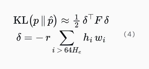
where the neurons are indexed in sorted order and we only keep the first 64Hₑ tiles of an expert when we read Hₑ tiles as compression. This is the quadratic form in the Fisher information that Optimal Brain Damage used to prune weights. Summing over the step’s tokens, we can split the cost of a read into two terms. The first term depends on the step, in particular on the number of tokens that use an expert and on the router weights of those tokens. The second term depends only on the stored model, in particular on the importance of the tiles that are skipped by the read.
Definition 2 (load and tail). The load of expert e in a step is Lₑ = Σ_(t→e) rₜ,ₑ². The importance of its tile k is Dₑ,ₖ = Σ_(i∈tile k) 𝔼[hᵢ²] wᵢᵀFwᵢ. The tail of a read of H tiles is tailₑ(H) = Σ_(k>H) Dₑ,ₖ.
The expected KL of a step’s cuts is thus given by the following equation.
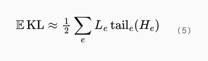
As we mentioned before, for other parts of the network the Fisher information F is roughly proportional to the number of hidden neurons I, so the importance of a tile is just the sum of the drop costs of the neurons in that tile. Thus, for each layer of each step we solve the following optimization problem:
Proposition 1 (water-filling). If Dₑ,ₖ is non-increasing in k and every tile costs the same bytes, a solution of Equation 6 reads from each expert exactly the tiles whose value clears one price λ ≥ 0:
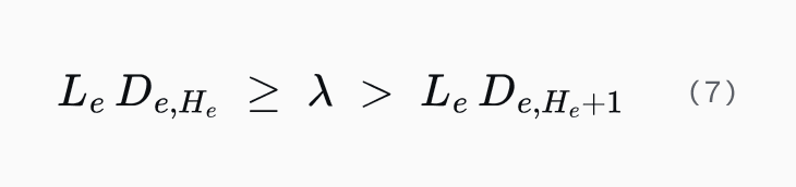
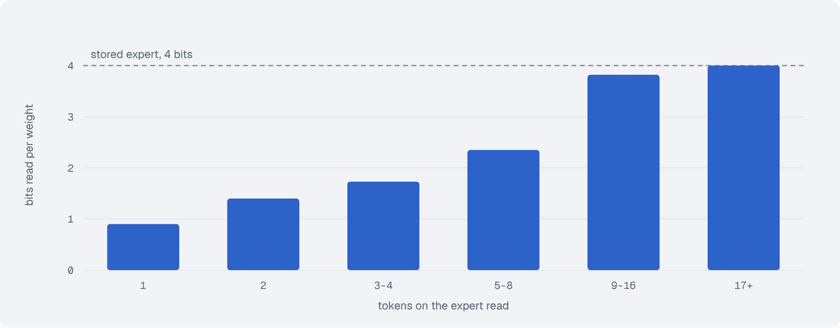
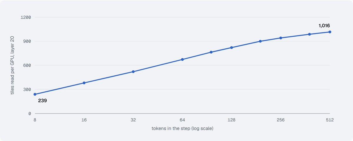
An expert with many tokens has a high load, so its tiles can be kept above the price until deep into the expert. An expert with only one token and a small router weight will be cut after a few tiles. Unlike a quantized model where the precision of each expert is fixed before the model is served, the precision of each read in a step can be derived from the tokens of that step. As a step grows in size, most of the extra tokens will land on experts that are already read, so the extra tokens will be read deeper into those experts, rather than as many new experts.
5. Load Balancing Between GPUs
On B300s we distribute the 384 experts of each layer over the 4 decode GPUs of that layer, so each GPU holds 96 of the experts of that layer. The memory read by the slowest GPU of a layer determines the memory read cost by the layer as a whole, so the budget in Equation 6 must hold on each GPU independently:
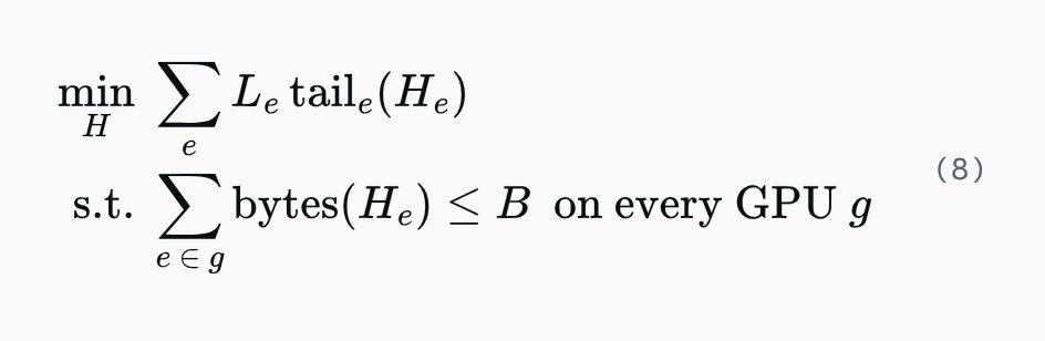
Proposition 2 (rank fill). The problem in Equation 8 can be solved for each GPU individually, and the solution for each GPU is a water-fill based on its price λ_g. Every GPU with tiles left to read spends its whole budget B.
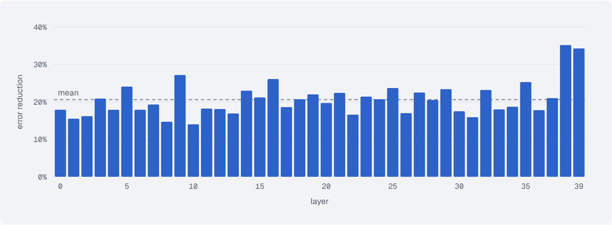
With a single price for the whole layer, every GPU except the busiest finishes its reads early and then sits idle. Instead we can use that time to read deeper into each GPU's own experts, which lowers the expected error on every layer. On a replay of served routing we solved Equation 8 for every step. The fixed budget that we serve comes out almost exactly as good as this oracle
7. How much does compression change the outputs?
Before we can talk about how much the compression of a model changes the output of that model, we must first determine how much the output of that model changes on a standard server without any compression. The original model does not reproduce exactly the same results on a standard server, because of the changes in floating point sums caused by the changes in the makeup of the batches of tokens that are processed by the server.
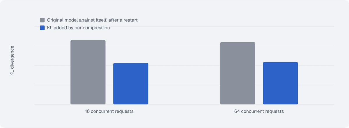
Definition 4 (restart floor). The restart floor is the KL between the original model and itself after server restart on the same set of requests in the same job as the compressed path.
We gate the KL added by compression on the restart floor. In every read the change added by compression is less than the change of the original model against itself (see Figure 13). The task scores on the path of compressed replies and the stock replies are within the intervals of each other, although the compressed replies are slightly longer than the stock replies and so are counted against speed in task pricing.
8. How bad can the worst reply get?
Since we're optimizing for a batch of users, we want to ensure a lower bound of quality degradation for any single user. A reasonable bound is to make the damage compression adds to any reply stay within the variance of the original model. Writing the KL of a reply along the compressed model's own outputs splits the damage into two parts, which we can bound separately:
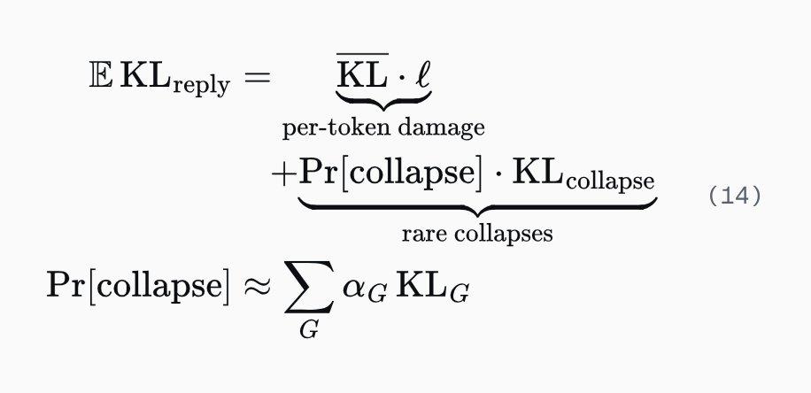
where ℓ is the reply length and KL_G the KL spent in layer group G. The first part is damage spread over a reply's tokens. The second is the rare reply that qualitatively collapses, at a rate that depends on where in the model the KL is spent rather than only on how much.
Definition 5 (worst-reply damage). The damage of a reply r is its mean KL per token, K̅L̅ᵣ = ℓᵣ⁻¹ Σ_(t∈r) KLₜ. The worst-reply damage of a deployment is the largest K̅L̅ᵣ among the replies it serves that do not collapse. Its collapse rate is the share of replies that do.
Damage per token at every step size. The expected damage per token for any step size T can be bounded by the budget of Section 4 for average damage per token over steps. However, a request decodes all of its tokens in steps of varying size depending on load, so a long reply decoded at peak load could have all of its tokens in the step size with the deepest cut. We therefore also cap the expected damage per token for any step size T:
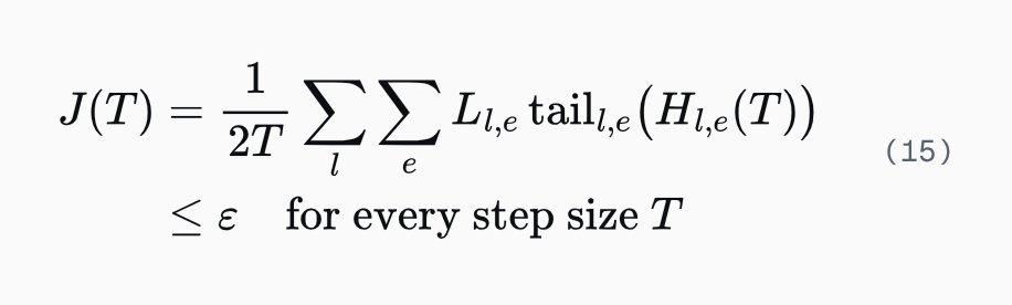
Each step size then solves Equation 6.
Spread of damage. Even though the average damage per token is bounded by the mean of a step, the damage can still be distributed very unevenly over the rows of a step. This is because the tiles of a read that are cut from a token’s reads depend on which experts the token picked. However, over a reply, the spread of damage over the rows of the steps is averaged down, because each consecutive token picks different experts. On served routing, the worst conversation of 60 tokens or more has 1.1-1.4x the mean damage of its steps (estimate). This is still well below the KL of a restart on an average reply.
Keeping track of each request. Each step can compute the tiles that it skips for each row of the step. The server can then keep a running tally of the total predicted damage for each request that has been served so far. After each token t of request r the server updates the total predicted damage for request r to Sᵣ ← max(0, Sᵣ + dₜ − ε), where dₜ is the predicted damage for token t by step size T. If Sᵣ is above h, then the server continues to read the experts that request uses deeper on all layers of the model, at least 12 tiles on every layer.
Proposition 5 (worst-reply bound). Suppose every token decoded while Sᵣ > h has predicted damage at most ε. Then a reply of n tokens that does not collapse has mean predicted damage at most ε + (h + dₘₐₓ)/n, where dₘₐₓ is the largest predicted damage of one token. Its true damage is at most 1 + δ times that, where δ bounds the relative error of the second-order model on a reply.
The excess over ε decreases with the length of a reply, so a long reply is held close to the cap itself. The cap of Equation 15 holds a typical request near ε, so the ledger only steps in for the few requests whose experts keep being cut deep.
Collapses. The second-order model cannot see a collapse, which is the second term of Equation 14. In served logs, though, the improbable tokens that mark a collapse begin to cluster hundreds of tokens before the reply turns into word salad, so an alarm on their density fires ahead of most collapses and on few healthy replies. An alarm that fires on 3 such tokens within 128 caught 168 of 186 collapsed replies, a median of 891 tokens before the onset, and fired on 0.70% of the 105,039 replies that did not collapse. A reply that raises the alarm can switch to whole reads for its remaining tokens.
Within variance. Each term of Equation 14 can then be held within variance of the original model. The damage of the worst reply should stay below the KL that a restart puts on an average reply, which it did empirically across benchmarks. The collapses that get past the alarm should be bounded by the rate at which the original model collapses.
9. How fast is it under load?
We can measure the speed of our entire stack of layers in two different ways. First, we can measure the throughput of the entire stack of layers by replaying the AgentX traces of InferenceX on a fleet of servers running in full mode (Table 6). Second, we can measure the speed of the entire stack of layers on InferenceX’s own agentic client at different loads. With one session, every expert read is used by exactly one token, so we read whole experts of a layer just like on stock servers. As the number of sessions increases, more tokens use each expert read, so setting the bytes of each expert read based on the number of tokens using that expert read saves more and more bytes compared with fixed-precision reading of all experts of a layer.
12. Conclusion
Starting from a second-order model of the KL that a cut adds, we worked out how many bytes a decode step should read to maximize throughput while keeping quality within variance of the original model.
If you serve open-weights models and want more out of the GPUs you already own, we would love to talk: dhruv@withsyzygy.com. We are also hiring researchers and engineers to work on problems like this one.